Two recently developed packages simplify programmatic access to LOBSTER data directly from your analysis environment:
R — lobsteR: Available on CRAN, lobsteR handles authentication, data requests, and downloads from the LOBSTER platform and integrates naturally with the highfrequency package for downstream analysis.
Python — lobsterdata: A lightweight Python client that lets you submit data construction requests, monitor their status, and download the resulting CSV files, covering the full asynchronous workflow of the LOBSTER API.
This exercise requires you mainly to familiarize yourself with LOBSTER, an online limit order book data tool that provides easy-to-use, high-quality data for the entire universe of NASDAQ traded stocks. I requested data based on their online interface and stored it on Absalon before running the code below. Lobster files contain all trading messages (order submissions, cancellations, trades) for a pre-specified ticker that went through NASDAQ. For example, the sample file in Absalon contains the entire order book history for the ticker SAP until level 5 in January 2022. LOBSTER generates a ‘message’ and an ‘orderbook’ file for each active trading day of a selected ticker. The ‘orderbook’ file contains the evolution of the limit order book up to the requested levels. The ‘message’ file contains indicators for the type of event causing an update of the limit order book in the requested price range. All events are time-stamped in seconds after midnight, with decimal precision of at least milliseconds and up to nanoseconds depending on the requested period.
The ‘message’ and ‘order book’ files are provided in the .csv format and can easily be read with any statistical software package.
Exercises:
Familiarize yourself with the output documentation of Lobster files on their homepage. Download the file SAP_2022-01-01_2022-01-31_5.7z from Absalon and read them using read_csv. Lobster files always have the same naming convention, ticker_date_34200000_57600000_filetype_level.csv, where filetype denotes message or the corresponding order book snapshots. Take notes on what you think are essential cleaning steps to get a helpful dataset comprising order book and trading information.
Merge the two files after you apply some intuitive naming convention such that you can work with one file which traces all information about messages and the corresponding order book snapshots. Try to create a function process_orderbook, which performs essential cleaning of the data by making sure you filter out trading halts and aggregate order execution messages which may have triggered multiple limit orders. More specifically, the function should complete the following generic steps:
Identify potential trading stops (consult the Lobster documentation for this) and discard all observations recorded during the window when trading was interrupted.
Sometimes, messages related to the daily opening and closing auction are included in the Lobster file (especially during days when trading stops earlier, e.g., before holidays). Remove such observations (opening auctions are identified as messages with type == 6 and ID == -1, and closing auctions can be identified as messages with type == 6 and ID == -2).
Replace “empty” slots in the order book with NAs in case there was no liquidity quoted at higher order book levels. In that case, Lobster reports negative bid and large ask prices (above 199999).
Remove observations with seemingly crossed prices (when the best ask is below the best bid).
Market orders are sometimes executed against multiple limit orders. In that case, Lobster records multiple transactions with an identical time stamp. Aggregate these transactions and generate the corresponding trade size and the (size-weighted) execution price. Also, retain the order book snapshot after the transaction has been executed.
The direction of a trade is hard to evaluate (not observable) if the transaction has been executed against a hidden order (type == 5). Create a proxy for the direction based on the executed price relative to the last observed order book snapshot.
You can use this function when you work with raw order book data from Lobster to produce a clean, analysis-ready order book. In the solution part, I provide some further explanations of my implementation. - Use the function to clean the SAP Lobster output. - Summarize the order book by extracting the average midquote \(q_t = (a_t + b_t)/2\) (where \(a_t\) and \(b_t\) denote the best bid and best ask), the average spread \(S_t= (a_t - b_t)/q_t\) (in basis points relative to the concurrent midquote), the aggregate volume in USD and the quoted depth (in million USD 5 basis points from the concurrent best price on each side of the order book) for each 5-minute interval.
- Provide a meaningful illustration of the order book dynamics during the particular trading day. This is intentionally a very open question: There is so much information within an order book that it is impossible to highlight everything worth considering. I encourage you to post your visualization on the discussion board in Absalon.
# A tibble: 40 × 5
   path                                                 size date   ticker level
   <chr>                                               <int> <chr>  <chr>  <chr>
 1 SAP_2022-01-28_34200000_57600000_message_5.csv          0 2022-… SAP    5
 2 SAP_2022-01-28_34200000_57600000_orderbook_5.csv        0 2022-… SAP    5
 3 SAP_2022-01-03_34200000_57600000_message_5.csv   14902108 2022-… SAP    5
 4 SAP_2022-01-03_34200000_57600000_orderbook_5.csv 38240040 2022-… SAP    5
 5 SAP_2022-01-04_34200000_57600000_message_5.csv   13248413 2022-… SAP    5
 6 SAP_2022-01-04_34200000_57600000_orderbook_5.csv 33881101 2022-… SAP    5
 7 SAP_2022-01-05_34200000_57600000_message_5.csv   12234669 2022-… SAP    5
 8 SAP_2022-01-05_34200000_57600000_orderbook_5.csv 31189574 2022-… SAP    5
 9 SAP_2022-01-06_34200000_57600000_message_5.csv   17311993 2022-… SAP    5
10 SAP_2022-01-06_34200000_57600000_orderbook_5.csv 44240752 2022-… SAP    5
# ℹ 30 more rows
Lobster files always follow the same naming convention; thus, the code above can be recycled in a more general fashion for other Lobster files. Next, we read in data for one(!) of the 20 trading days.
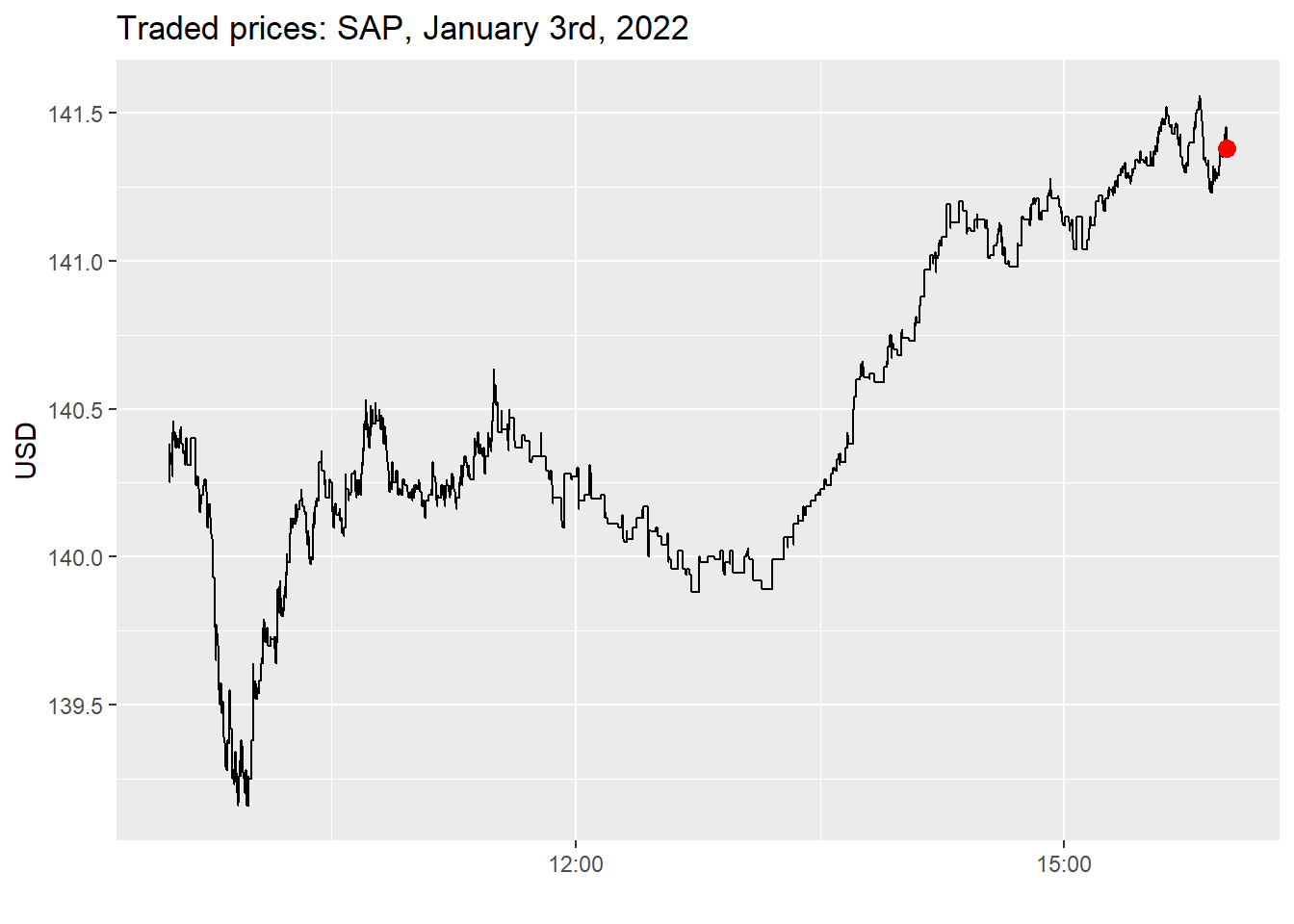
messages_raw <-read_csv( archive::archive_read("SAP_2022-01-01_2022-01-31_5.7z", 3),col_names =c("ts","type","order_id","m_size","m_price","direction","null" ),col_type =cols(null =col_skip())) |>mutate(ts =as.POSIXct( ts,origin =as.Date("2022-01-07"),tz ="GMT",format ="%Y-%m-%d %H:%M:%OS6" ),m_price = m_price /10000 )messages_raw |>filter(type ==4| type ==5) |>ggplot(aes(x = ts, y = m_price)) +geom_step() +geom_point(data = messages_raw |>tail(1), color ="red", size =3) +labs(x ="", y ="USD", title ="Traded prices: SAP, January 3rd, 2022")
Figure 1: Traded prices for SAP on January 3rd, 2022, based on execution messages (types 4 and 5).
Note my naming convention for column names. The command col_type makes sure that there is easy processing afterward. By default, ts denotes the time in seconds since midnight (decimals are precise until the nanosecond level), and price always comes in 10.000 USD. type denotes the message type: 4, for instance, corresponds to the execution of a visible order. The remaining variables are explained in more detail here.
Next, the corresponding orderbook snapshots contain price and quoted size for each of the 5 levels.
Each message is associated with the corresponding order book snapshot. After merging the message and orderbook files, the entire data thus looks as follows.
The code below is rather flexible to handle Lobster files with more or less levels. Each column contains the corresponding prices and sizes on each side of the order book. More information is available on the documentation of Lobster. The output contains one file with all information available in the order book.
The order book contains 316379 observations. While the columns ts to direction help understand the specific messages, the remaining columns contain a snapshot of the order book at that particular time.
Next, Lobster sometimes contains opening and closing auctions (in particular on days when trading hours deviate from the regular times). If you follow the documentation on Lobster, you will see that these times can be identified as I do in the code below.
In line with the exercise, the function process_orderbook() performs several essential steps. You can call it from within R with the following command.
process_orderbook <-function(orderbook) {# Did a trading halt happen? ---- halt_index <- orderbook |>filter( type ==7& direction ==-1& m_price ==-1/10000| type ==7& direction ==-1& m_price ==1/10000 )while (nrow(halt_index) >1) {# Filter out messages that occurred in between trading haltscat("Trading halt detected") orderbook <- orderbook |>filter(ts < halt_index$ts[1] | ts > halt_index$ts[2]) halt_index <- halt_index |>filter(row_number() >2) }# Opening and closing auction ----# Discard everything before type 6 & ID -1 and everything after type 6 & ID -2 opening_auction <- orderbook |>filter( type ==6, order_id ==-1 ) |>pull(ts) closing_auction <- orderbook |>filter( type ==6, order_id ==-2 ) |>pull(ts)if (length(opening_auction) !=1) { opening_auction <- orderbook |>select(ts) |>head(1) |>pull(ts) - lubridate::seconds(0.1) }if (length(closing_auction) !=1) { closing_auction <- orderbook |>select(ts) |>tail(1) |>pull(ts) + lubridate::seconds(0.1) } orderbook <- orderbook |>filter(ts > opening_auction & ts < closing_auction) orderbook <- orderbook |>filter(type !=6& type !=7)# Replace "empty" slots in the order book (0 volume) with NA prices ---- orderbook <- orderbook |>mutate(across(contains("bid_price"), ~replace(., . <0, NA)),across(contains("ask_price"), ~replace(., . >=999999, NA)) )# Remove crossed order book observations ---- orderbook <- orderbook |>filter(ask_price_1 > bid_price_1)# Merge transactions with unique timestamp ---- trades <- orderbook |>filter(type ==4| type ==5) |>select(ts:direction) trades <-inner_join( trades, orderbook |>group_by(ts) |>filter(row_number() ==1) |>ungroup() |>transmute( ts, ask_price_1, bid_price_1,midquote = ask_price_1 /2+ bid_price_1 /2,lag_midquote =lag(midquote) ),by ="ts" ) trades <- trades |>mutate(direction =case_when( type ==5& m_price < lag_midquote ~1, # lobster convention: direction = 1 if executed against a limit buy order type ==5& m_price > lag_midquote ~-1, type ==4~as.double(direction),TRUE~as.double(NA) ) )# Aggregate transactions with size and volume-weighted price trade_aggregated <- trades |>group_by(ts) |>summarise(type =last(type),order_id =NA,m_price =sum(m_price * m_size) /sum(m_size),m_size =sum(m_size),direction =last(direction) )# Merge trades with the last observed order book snapshot trade_aggregated <-inner_join( trade_aggregated, orderbook |>select(ts, ask_price_1:last_col()) |>group_by(ts) |>filter(row_number() ==n()),by ="ts" ) orderbook <- orderbook |>filter( type !=4, type !=5 ) |>bind_rows(trade_aggregated) |>arrange(ts) |>mutate(direction =if_else(type ==4| type ==5, direction, as.double(NA)))return(orderbook)}
You can process the raw data from before by simply calling.
orderbook <-process_orderbook(orderbook)
The function compute_depth below computes the number of traded shares within bp basis points of the associated best price, which can be used to measure liquidity.
compute_depth <-function(orderbook, side ="bid", bp =0) {# Computes depth (in contracts) based on order book snapshotsif (side =="bid") { value_bid <- (1- bp /10000) * orderbook |>select("bid_price_1") index_bid <- orderbook |>select(contains("bid_price")) |>mutate_all(function(x) {if_else(is.na(x), FALSE, x >= value_bid) }) sum_vector <- (orderbook |>select(contains("bid_size")) * index_bid) |>rowSums(na.rm =TRUE) } else { value_ask <- (1+ bp /10000) * orderbook |>select("ask_price_1") index_ask <- orderbook |>select(contains("ask_price")) |>mutate_all(function(x) {if_else(is.na(x), FALSE, x <= value_ask) }) sum_vector <- (orderbook |>select(contains("ask_size")) * index_ask) |>rowSums(na.rm =TRUE) }return(sum_vector)}
Next, I compute the midquote, bid-ask spread, aggregate volume, and depth (the amount of trade-able units in the order book):
Midquote \(q_t = (a_t + b_t)/2\) (where \(a_t\) and \(b_t\) denote the best bid and best ask)
Spread \(S_t= (a_t - b_t)\) (values below are computed in basis points relative to the concurrent midquote)
Volume is the aggregate sum of traded units of the stock. I do not differentiate between hidden (type==5) and visible volume.
Depth at the best level.
I aggregate the information into buckets of 5 minutes, using time-weighting for the order book variables.
Five-minute summaries of midquote, spread (bps), trade count, volume, and quoted depth for SAP, January 2022.
Time
Order book
Trading activity
Midquote (USD)
Spread (bps)
Bid depth
Ask depth
Trades
Messages
Volume (USD)
9:30 AM
$140.38
3.62
485
534
61
12,926
$1,313,466
9:35 AM
$140.24
4.33
669
584
23
14,844
$602,060
9:40 AM
$140.15
4.31
761
427
24
11,150
$299,088
9:45 AM
$139.49
4.54
777
557
43
12,891
$711,751
9:50 AM
$139.26
4.76
713
720
45
20,975
$643,746
9:55 AM
$139.31
4.79
748
628
46
17,916
$666,569
10:00 AM
$139.81
5.05
749
671
37
17,288
$640,948
10:05 AM
$139.81
4.93
835
520
42
14,336
$517,071
10:10 AM
$140.16
5.33
805
796
32
11,862
$609,344
10:15 AM
$140.17
4.59
493
633
24
11,218
$218,798
10:20 AM
$140.25
4.31
567
652
69
10,213
$1,392,951
10:25 AM
$140.18
4.54
470
805
17
12,386
$193,138
10:30 AM
$140.19
4.43
447
715
27
12,563
$443,163
10:35 AM
$140.29
3.61
435
426
44
10,616
$408,664
10:40 AM
$140.49
4.04
554
548
91
10,862
$1,516,834
10:45 AM
$140.43
4.51
467
758
28
12,057
$249,738
10:50 AM
$140.24
4.32
407
746
36
11,627
$292,742
10:55 AM
$140.21
3.61
299
787
19
8,978
$363,035
11:00 AM
$140.18
2.79
178
950
45
8,117
$852,378
11:05 AM
$140.19
4.07
455
821
29
8,625
$788,170
11:10 AM
$140.23
3.13
366
513
57
9,471
$1,794,017
11:15 AM
$140.31
2.79
278
470
36
9,019
$547,094
11:20 AM
$140.37
3.72
528
594
40
7,751
$742,033
11:25 AM
$140.57
4.10
526
533
58
12,209
$1,843,627
11:30 AM
$140.39
6.24
219
522
47
2,706
$1,043,222
11:35 AM
$140.37
8.53
240
203
41
501
$926,211
11:40 AM
$140.37
8.63
173
166
16
207
$82,531
11:45 AM
$140.31
5.78
136
188
19
212
$201,726
11:50 AM
$140.14
6.04
82
56
10
405
$111,357
11:55 AM
$140.25
6.20
154
170
12
398
$142,420
12:00 PM
$140.22
6.09
138
119
10
234
$143,158
12:05 PM
$140.23
6.90
142
46
14
188
$171,964
12:10 PM
$140.13
5.57
188
72
14
157
$129,363
12:15 PM
$140.08
3.55
109
68
17
192
$191,348
12:20 PM
$140.17
3.94
120
44
9
143
$63,614
12:25 PM
$140.10
4.88
134
121
21
210
$173,409
12:30 PM
$140.00
6.99
138
165
26
286
$407,699
12:35 PM
$140.00
5.66
50
121
32
300
$586,622
12:40 PM
$139.94
5.94
229
76
8
198
$82,985
12:45 PM
$139.99
5.80
210
79
10
188
$27,437
12:50 PM
$139.94
4.92
288
103
13
255
$122,189
12:55 PM
$139.99
4.16
171
113
6
257
$59,784
1:00 PM
$139.95
4.83
255
167
13
240
$168,846
1:05 PM
$139.91
6.02
152
142
2
137
$6,995
1:10 PM
$140.07
7.01
192
122
3
310
$19,176
1:15 PM
$140.06
6.59
162
221
5
139
$21,009
1:20 PM
$140.17
3.50
213
26
10
189
$84,217
1:25 PM
$140.21
2.68
250
156
9
147
$79,495
1:30 PM
$140.28
2.34
237
100
12
196
$112,770
1:35 PM
$140.39
3.00
172
120
26
340
$322,772
1:40 PM
$140.63
6.59
274
88
18
483
$121,353
1:45 PM
$140.62
4.52
106
126
17
247
$172,959
1:50 PM
$140.68
5.11
251
71
7
178
$40,787
1:55 PM
$140.72
4.62
168
153
17
270
$193,457
2:00 PM
$140.75
4.61
285
150
10
127
$72,340
2:05 PM
$140.97
6.84
398
196
16
348
$154,616
2:10 PM
$141.11
4.68
278
110
32
285
$362,107
2:15 PM
$141.18
4.06
191
146
14
283
$176,133
2:20 PM
$141.12
2.63
129
125
25
375
$242,762
2:25 PM
$141.13
4.58
139
61
17
204
$196,725
2:30 PM
$141.03
3.71
183
74
12
201
$77,879
2:35 PM
$141.01
4.19
170
46
30
406
$330,383
2:40 PM
$141.19
8.42
163
88
11
247
$142,360
2:45 PM
$141.20
4.63
391
48
17
240
$155,433
2:50 PM
$141.24
5.42
297
86
27
358
$381,499
2:55 PM
$141.12
3.00
87
76
23
492
$263,047
3:00 PM
$141.14
5.22
145
147
19
577
$123,330
3:05 PM
$141.12
3.25
173
124
14
285
$199,390
3:10 PM
$141.20
2.59
303
19
23
430
$332,351
3:15 PM
$141.29
2.48
218
137
41
600
$451,828
3:20 PM
$141.29
2.08
181
174
56
517
$806,482
3:25 PM
$141.33
1.74
287
111
39
582
$559,393
3:30 PM
$141.44
2.30
198
117
64
1,028
$739,473
3:35 PM
$141.44
2.13
263
111
65
864
$886,603
3:40 PM
$141.29
2.51
206
103
57
1,252
$742,247
3:45 PM
$141.56
2.84
355
165
35
1,065
$242,671
3:50 PM
$141.29
2.50
193
151
154
2,458
$2,367,376
3:55 PM
$141.43
2.00
246
161
140
2,142
$1,857,272
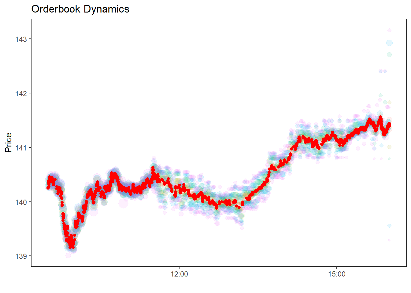
Finally, some visualization of the data at hand: The code below shows the dynamics of the traded prices (red points) and the quoted prices at the higher order book levels.
I use the following code to read in (general) Lobster files - change ticker, date, and level in the code snippet below.
archive_path ="SAP_2022-01-01_2022-01-31_5.7z"with py7zr.SevenZipFile(archive_path, mode="r") as archive: file_info = archive.list()files_available = pd.DataFrame( {"path": [f.filename for f in file_info], "size": [f.uncompressed for f in file_info]})files_available[["ticker", "date", "level"]] = ( files_available["path"].str.extract(r"(.*)_(.*)_342.*_(.*).csv"))files_available.head(10)
path
size
ticker
date
level
0
SAP_2022-01-28_34200000_57600000_message_5.csv
0
SAP
2022-01-28
5
1
SAP_2022-01-28_34200000_57600000_orderbook_5.csv
0
SAP
2022-01-28
5
2
SAP_2022-01-03_34200000_57600000_message_5.csv
14902108
SAP
2022-01-03
5
3
SAP_2022-01-03_34200000_57600000_orderbook_5.csv
38240040
SAP
2022-01-03
5
4
SAP_2022-01-04_34200000_57600000_message_5.csv
13248413
SAP
2022-01-04
5
5
SAP_2022-01-04_34200000_57600000_orderbook_5.csv
33881101
SAP
2022-01-04
5
6
SAP_2022-01-05_34200000_57600000_message_5.csv
12234669
SAP
2022-01-05
5
7
SAP_2022-01-05_34200000_57600000_orderbook_5.csv
31189574
SAP
2022-01-05
5
8
SAP_2022-01-06_34200000_57600000_message_5.csv
17311993
SAP
2022-01-06
5
9
SAP_2022-01-06_34200000_57600000_orderbook_5.csv
44240752
SAP
2022-01-06
5
Lobster files always follow the same naming convention; thus, the code above can be recycled in a more general fashion for other Lobster files. The helper below extracts a single file from the archive into memory, mirroring archive::archive_read() in R.
<plotnine.ggplot.ggplot object at 0x00000233BAD70E50>
Note my naming convention for column names. The argument usecols=range(6) makes sure we drop the trailing null column for easy processing afterward. By default, ts denotes the time in seconds since midnight (decimals are precise until the nanosecond level), and price always comes in 10.000 USD. type denotes the message type: 4, for instance, corresponds to the execution of a visible order. The remaining variables are explained in more detail here.
Next, the corresponding orderbook snapshots contain price and quoted size for each of the 5 levels.
The code below is rather flexible to handle Lobster files with more or less levels. Each column contains the corresponding prices and sizes on each side of the order book. After merging the message and orderbook files, the entire data thus looks as follows.
level =5ob_cols = [f"{var}_{lvl}"for lvl inrange(1, level +1)for var in ("ask_price", "ask_size", "bid_price", "bid_size")]orderbook_raw = read_archive_csv(archive_path, target_index=3, names=ob_cols)price_cols = [c for c in orderbook_raw.columns if"price"in c]orderbook_raw[price_cols] = orderbook_raw[price_cols] /10000orderbook = pd.concat( [messages_raw.reset_index(drop=True), orderbook_raw.reset_index(drop=True)], axis=1,)pd.set_option("display.max_columns", 7)orderbook.head(10)
ts
type
order_id
...
ask_size_5
bid_price_5
bid_size_5
0
2022-01-03 09:30:00.041693104+00:00
3
34351556
...
696
140.23
800
1
2022-01-03 09:30:00.042287443+00:00
1
34456580
...
696
140.23
800
2
2022-01-03 09:30:00.042327460+00:00
3
34390184
...
764
140.23
800
3
2022-01-03 09:30:00.043255366+00:00
1
34457908
...
764
140.23
800
4
2022-01-03 09:30:00.043453093+00:00
3
34302936
...
764
140.23
800
5
2022-01-03 09:30:00.043699050+00:00
1
34458304
...
764
140.23
800
6
2022-01-03 09:30:00.049983479+00:00
3
34457908
...
764
140.23
800
7
2022-01-03 09:30:00.050566166+00:00
1
34463304
...
696
140.23
800
8
2022-01-03 09:30:00.050704660+00:00
2
34458304
...
696
140.23
800
9
2022-01-03 09:30:00.051073967+00:00
2
34458304
...
696
140.23
800
10 rows × 26 columns
The order book contains as many observations as the message file. While the columns ts to direction help understand the specific messages, the remaining columns contain a snapshot of the order book at that particular time.
Next, Lobster sometimes contains opening and closing auctions (in particular on days when trading hours deviate from the regular times). If you follow the documentation on Lobster, you will see that these times can be identified as I do in the code below.
In line with the exercise, the function process_orderbook() performs several essential steps. You can call it from within Python with the following command.
def process_orderbook(orderbook): orderbook = orderbook.copy()# Did a trading halt happen? ---- halt_mask = ( (orderbook["type"] ==7)& (orderbook["direction"] ==-1)& (orderbook["m_price"].isin([-1/10000, 1/10000])) ) halt_ts = orderbook.loc[halt_mask, "ts"].reset_index(drop=True)whilelen(halt_ts) >1:# Filter out messages that occurred in between trading haltsprint("Trading halt detected") orderbook = orderbook[ (orderbook["ts"] < halt_ts.iloc[0]) | (orderbook["ts"] > halt_ts.iloc[1]) ] halt_ts = halt_ts.iloc[2:].reset_index(drop=True)# Opening and closing auction ----# Discard everything before type 6 & ID -1 and everything after type 6 & ID -2 opening = orderbook.loc[ (orderbook["type"] ==6) & (orderbook["order_id"] ==-1), "ts" ] closing = orderbook.loc[ (orderbook["type"] ==6) & (orderbook["order_id"] ==-2), "ts" ] open_ts = ( opening.iloc[0]iflen(opening) ==1else orderbook["ts"].iloc[0] - pd.Timedelta("0.1s") ) close_ts = ( closing.iloc[0]iflen(closing) ==1else orderbook["ts"].iloc[-1] + pd.Timedelta("0.1s") ) orderbook = orderbook[(orderbook["ts"] > open_ts) & (orderbook["ts"] < close_ts)] orderbook = orderbook[~orderbook["type"].isin([6, 7])]# Replace "empty" slots in the order book (0 volume) with NA prices ---- bid_price_cols = [c for c in orderbook.columns if"bid_price"in c] ask_price_cols = [c for c in orderbook.columns if"ask_price"in c] orderbook[bid_price_cols] = orderbook[bid_price_cols].mask(orderbook[bid_price_cols] <0) orderbook[ask_price_cols] = orderbook[ask_price_cols].mask(orderbook[ask_price_cols] >=999999)# Remove crossed order book observations ---- orderbook = orderbook[orderbook["ask_price_1"] > orderbook["bid_price_1"]]# Merge transactions with unique timestamp ---- trades = orderbook[orderbook["type"].isin([4, 5])][ ["ts", "type", "order_id", "m_size", "m_price", "direction"] ].copy() snapshots = ( orderbook.drop_duplicates(subset="ts", keep="first") .assign(midquote=lambda d: (d["ask_price_1"] + d["bid_price_1"]) /2) [["ts", "ask_price_1", "bid_price_1", "midquote"]] .sort_values("ts") .reset_index(drop=True) ) snapshots["lag_midquote"] = snapshots["midquote"].shift(1) trades = trades.merge(snapshots, on="ts", how="inner")# lobster convention: direction = 1 if executed against a limit buy order trades["direction"] = np.where( (trades["type"] ==5) & (trades["m_price"] < trades["lag_midquote"]),1.0, np.where( (trades["type"] ==5) & (trades["m_price"] > trades["lag_midquote"]),-1.0, np.where(trades["type"] ==4, trades["direction"].astype(float), np.nan), ), )# Aggregate transactions with size and volume-weighted price trade_aggregated = trades.groupby("ts", as_index=False).apply(lambda g: pd.Series( {"type": g["type"].iloc[-1],"order_id": np.nan,"m_price": np.sum(g["m_price"] * g["m_size"]) / g["m_size"].sum(),"m_size": g["m_size"].sum(),"direction": g["direction"].iloc[-1], } ), include_groups=False, )# Merge trades with the last observed order book snapshot snapshot_cols = ["ts"] + [ c for c in orderbook.columns if c.startswith(("ask_", "bid_")) ] last_snapshot = ( orderbook[snapshot_cols] .drop_duplicates(subset="ts", keep="last") .reset_index(drop=True) ) trade_aggregated = trade_aggregated.merge(last_snapshot, on="ts", how="inner") non_trades = orderbook[~orderbook["type"].isin([4, 5])] orderbook = ( pd.concat([non_trades, trade_aggregated], ignore_index=True) .sort_values("ts") .reset_index(drop=True) ) orderbook["direction"] = np.where( orderbook["type"].isin([4, 5]), orderbook["direction"], np.nan )return orderbook
You can process the raw data from before by simply calling.
orderbook = process_orderbook(orderbook)
The function compute_depth below computes the number of traded shares within bp basis points of the associated best price, which can be used to measure liquidity.
def compute_depth(orderbook, side="bid", bp=0):# Computes depth (in contracts) based on order book snapshotsif side =="bid": ref = (1- bp /10000) * orderbook["bid_price_1"] price_cols = [c for c in orderbook.columns if"bid_price"in c] size_cols = [c for c in orderbook.columns if"bid_size"in c] idx = orderbook[price_cols].ge(ref, axis=0).fillna(False)else: ref = (1+ bp /10000) * orderbook["ask_price_1"] price_cols = [c for c in orderbook.columns if"ask_price"in c] size_cols = [c for c in orderbook.columns if"ask_size"in c] idx = orderbook[price_cols].le(ref, axis=0).fillna(False) sizes = orderbook[size_cols].fillna(0).valuesreturn (sizes * idx.values).sum(axis=1)
Next, I compute the midquote, bid-ask spread, aggregate notional volume, and depth (the amount of trade-able units in the order book):
Midquote \(q_t = (a_t + b_t)/2\) (where \(a_t\) and \(b_t\) denote the best bid and best ask)
Spread \(S_t= (a_t - b_t)\) (values below are computed in basis points relative to the concurrent midquote)
Notional volume is the aggregate traded dollar value of the stock, computed as trade price times trade size. I do not differentiate between hidden (type==5) and visible trade volume.
Depth at the best level.
I aggregate the information into buckets of 5 minutes, using time-weighting for the order book variables.
Table 1: Five-minute summaries of midquote, spread (bps), trade count, notional volume, and quoted depth for SAP, January 2022.
Time
Order book
Trading activity
Midquote (USD)
Spread (bps)
Bid depth
Ask depth
Trades
Messages
Volume (USD)
9:30 AM
$140.38
3.62
482
533
61
12,926
$1,313,466
9:35 AM
$140.24
4.33
668
583
23
14,844
$602,060
9:40 AM
$140.15
4.32
760
424
24
11,150
$299,088
9:45 AM
$139.49
4.54
776
554
43
12,891
$711,751
9:50 AM
$139.26
4.76
711
717
45
20,975
$643,746
9:55 AM
$139.31
4.79
747
626
46
17,916
$666,569
10:00 AM
$139.81
5.05
747
671
37
17,288
$640,948
10:05 AM
$139.81
4.93
831
518
42
14,336
$517,071
10:10 AM
$140.16
5.33
804
795
32
11,862
$609,344
10:15 AM
$140.17
4.59
491
633
24
11,218
$218,798
10:20 AM
$140.25
4.31
566
651
69
10,213
$1,392,951
10:25 AM
$140.18
4.55
469
804
17
12,386
$193,138
10:30 AM
$140.19
4.44
446
714
27
12,563
$443,163
10:35 AM
$140.29
3.61
431
426
44
10,616
$408,664
10:40 AM
$140.49
4.04
551
547
91
10,862
$1,516,834
10:45 AM
$140.43
4.51
466
756
28
12,057
$249,738
10:50 AM
$140.24
4.32
405
745
36
11,627
$292,742
10:55 AM
$140.21
3.61
299
787
19
8,978
$363,035
11:00 AM
$140.18
2.79
178
950
45
8,117
$852,378
11:05 AM
$140.19
4.08
448
819
29
8,625
$788,170
11:10 AM
$140.23
3.13
363
510
57
9,471
$1,794,017
11:15 AM
$140.31
2.79
277
470
36
9,019
$547,094
11:20 AM
$140.37
3.72
527
593
40
7,751
$742,033
11:25 AM
$140.57
4.10
525
528
58
12,209
$1,843,627
11:30 AM
$140.39
6.24
219
522
47
2,706
$1,043,222
11:35 AM
$140.37
8.53
240
203
41
501
$926,211
11:40 AM
$140.37
8.63
173
166
16
207
$82,531
11:45 AM
$140.31
5.78
136
188
19
212
$201,726
11:50 AM
$140.14
6.04
82
56
10
405
$111,357
11:55 AM
$140.25
6.20
154
170
12
398
$142,420
12:00 PM
$140.22
6.09
138
119
10
234
$143,158
12:05 PM
$140.23
6.90
142
46
14
188
$171,964
12:10 PM
$140.13
5.57
188
72
14
157
$129,363
12:15 PM
$140.08
3.55
109
68
17
192
$191,348
12:20 PM
$140.17
3.94
120
44
9
143
$63,614
12:25 PM
$140.10
4.88
134
121
21
210
$173,409
12:30 PM
$140.00
6.99
138
165
26
286
$407,699
12:35 PM
$140.00
5.66
50
121
32
300
$586,622
12:40 PM
$139.94
5.94
229
76
8
198
$82,985
12:45 PM
$139.99
5.80
210
79
10
188
$27,437
12:50 PM
$139.94
4.92
288
103
13
255
$122,189
12:55 PM
$139.99
4.16
171
113
6
257
$59,784
1:00 PM
$139.95
4.83
255
167
13
240
$168,846
1:05 PM
$139.91
6.02
152
142
2
137
$6,995
1:10 PM
$140.07
7.01
192
122
3
310
$19,176
1:15 PM
$140.06
6.59
162
221
5
139
$21,009
1:20 PM
$140.17
3.50
213
26
10
189
$84,217
1:25 PM
$140.21
2.68
250
156
9
147
$79,495
1:30 PM
$140.28
2.34
237
100
12
196
$112,770
1:35 PM
$140.39
3.00
172
120
26
340
$322,772
1:40 PM
$140.63
6.59
274
88
18
483
$121,353
1:45 PM
$140.62
4.52
106
126
17
247
$172,959
1:50 PM
$140.68
5.11
251
71
7
178
$40,787
1:55 PM
$140.72
4.62
168
153
17
270
$193,457
2:00 PM
$140.75
4.61
285
150
10
127
$72,340
2:05 PM
$140.97
6.84
398
196
16
348
$154,616
2:10 PM
$141.11
4.68
278
110
32
285
$362,107
2:15 PM
$141.18
4.06
190
146
14
283
$176,133
2:20 PM
$141.12
2.63
129
125
25
375
$242,762
2:25 PM
$141.13
4.58
139
61
17
204
$196,725
2:30 PM
$141.03
3.71
183
74
12
201
$77,879
2:35 PM
$141.01
4.19
170
46
30
406
$330,383
2:40 PM
$141.19
8.42
163
88
11
247
$142,360
2:45 PM
$141.20
4.63
391
48
17
240
$155,433
2:50 PM
$141.24
5.42
297
86
27
358
$381,499
2:55 PM
$141.12
3.00
87
76
23
492
$263,047
3:00 PM
$141.14
5.22
144
147
19
577
$123,330
3:05 PM
$141.12
3.25
173
124
14
285
$199,390
3:10 PM
$141.20
2.59
303
19
23
430
$332,351
3:15 PM
$141.29
2.48
218
137
41
600
$451,828
3:20 PM
$141.29
2.08
181
174
56
517
$806,482
3:25 PM
$141.33
1.74
287
111
39
582
$559,393
3:30 PM
$141.44
2.30
198
117
64
1,028
$739,473
3:35 PM
$141.44
2.13
263
111
65
864
$886,603
3:40 PM
$141.29
2.51
206
103
57
1,252
$742,247
3:45 PM
$141.56
2.84
355
165
35
1,065
$242,671
3:50 PM
$141.29
2.50
193
151
154
2,458
$2,367,376
3:55 PM
$141.43
2.00
246
161
140
2,142
$1,857,272
Finally, some visualization of the data at hand: The code below shows the dynamics of the traded prices (red points) and the quoted prices at the higher order book levels.
<plotnine.ggplot.ggplot object at 0x00000233BB62F090>
Brownian Motion and realized volatility
In this exercise, you will analyze the empirical properties of the (geometric) Brownian motion based on a simulation study. Such simulation studies can also be helpful for various applications in continuous time finance, e.g., option pricing.
Finance theory suggests that prices must be so-called semimartingales. The most commonly used semimartingale is the Geometric Brownian Motion (GBM), where we assume that the logarithm of the stock price \(S_t\), \(X_t = \log(S_t)\) follows the following dynamic \[
X_t = X_0 + \mu t + \sigma W_t
\] where \(\mu\) and \(\sigma\) are constants and \(W_t\) is a Brownian motion.
Exercises:
Write a function that simulates (log) stock prices according to the model above. Recall that the Brownian motion has independent increments which are normally distributed. The function should generate a path of the log stock price with a pre-defined number of observations (granularity), drift term, and volatility. Then, plot one sample path of the implied (log) stock price.
Use the function to simulate a large number of geometric Brownian motions. Illustrate the quadratic variation of the process.
Compute the realized volatility for each simulated process and illustrate the sampling distribution.
Finally, consider the infill asymptotics. Show the effect of sampling once per day, once per hour, once per minute, and so on on the variance of the realized volatility.
For this exercise, I use some functionalities from the xts and highfrequency packages, particularly for aggregation at different frequencies.
library(dplyr)library(tidyr)library(xts)
Loading required package: zoo
Attaching package: 'zoo'
The following objects are masked from 'package:base':

    as.Date, as.Date.numeric
######################### Warning from 'xts' package ##########################
#                                                                             #
# The dplyr lag() function breaks how base R's lag() function is supposed to  #
# work, which breaks lag(my_xts). Calls to lag(my_xts) that you type or       #
# source() into this session won't work correctly.                            #
#                                                                             #
# Use stats::lag() to make sure you're not using dplyr::lag(), or you can add #
# conflictRules('dplyr', exclude = 'lag') to your .Rprofile to stop           #
# dplyr from breaking base R's lag() function.                                #
#                                                                             #
# Code in packages is not affected. It's protected by R's namespace mechanism #
# Set `options(xts.warn_dplyr_breaks_lag = FALSE)` to suppress this warning.  #
#                                                                             #
###############################################################################
Attaching package: 'xts'
The following objects are masked from 'package:dplyr':

    first, last
library(highfrequency)
Warning: package 'highfrequency' was built under R version 4.5.3
library(purrr)library(ggplot2)library(lubridate)
Note: When loading xts and the tidyverse jointly, you may run into serious issues if you do not consider naming conflicts! Especially the convenient functions last and first from dplyr may be affected. For that purpose, I consistently use dplyr::first and dplyr::last in this chapter.
First, the function below is a rather general version of a simulated generalized Brownian motion. Note that there is no immediate need to assign trading date and hour; I implement this because it will provide output closer to actual data, and therefore, parts of my code can be recycled for future projects. The function can be called with a specific seed to replicate the results. The relevant parameters are the initial values start and the geometric Brownian motion mu and sigma parameters. The input steps defines the simulated Brownian motion’s granularity (sampling frequency).
Note the last line of the function doing most of the work: We exploit that increments of a Brownian motion are independent and normally distributed. The entire path is nothing but the cumulative sum of the increments.
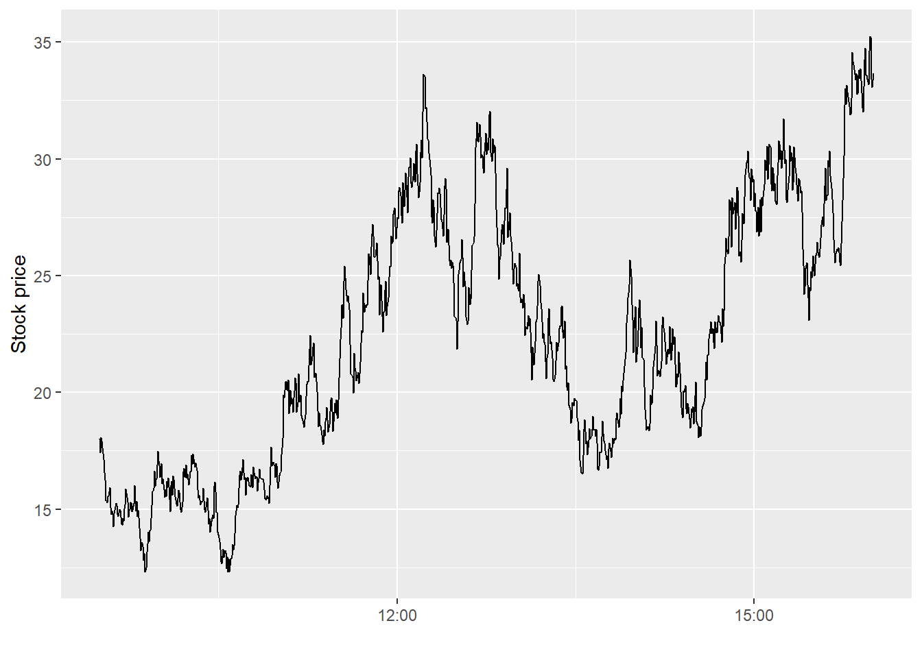
Next, I simulate the stock price with 1000 intraday observations. Recall that the geometric Brownian motion implies dynamics for the log of the stock price, which is why I adjust the plotted value in the \(y\)-axis.
tab <-simulate_geom_brownian_motion(start =log(18))tab |>ggplot(aes(x = time, y =exp(price))) +geom_line() +labs(x ="", y ="Stock price")
Figure 3: A single simulated intraday path of the geometric Brownian motion (1000 steps).
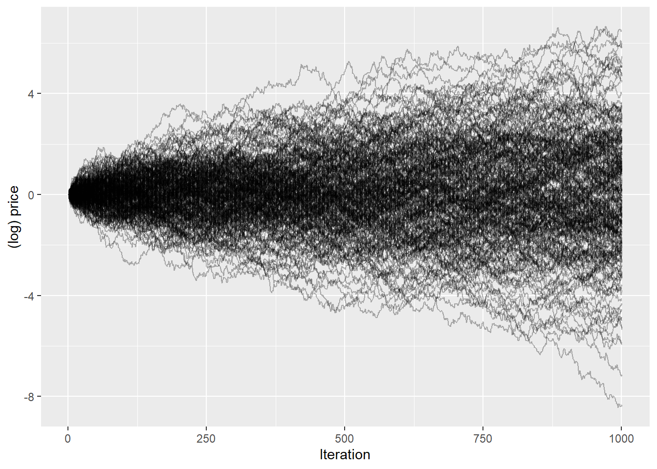
Next, we scale the simulation up. The code below simulates 250 paths of the geometric Brownian motion, all with the same starting value. The function illustrates the sampled (log) price paths.
Figure 4: Two hundred and fifty simulated log price paths of the geometric Brownian motion (\(\sigma = 2.4\), 1000 intraday steps each).
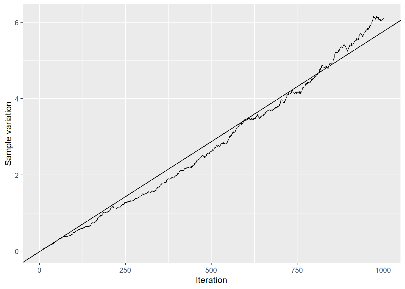
Next, we investigate some of the properties of the geometric Brownian motion. First, by definition, the sample variation of \(X_t = \int\limits_0^t\mu dt + \int\limits_0^t\sigma dW_t\) is \(\int\limits_0^t\sigma^2 dt = \sigma^2t\). The figure below illustrates the sample variation over time and shows that the standard deviation across all simulated (log) prices increases linearly in \(t\) as expected. For the simulation, I used \(\sigma = 2.4\) (true_sigma), which corresponds to the slope of the line (adjusted by the number of observations).
Figure 5: Sample variation of simulated GBM log prices over time; the straight line shows the theoretical \(\sigma^2 t\).
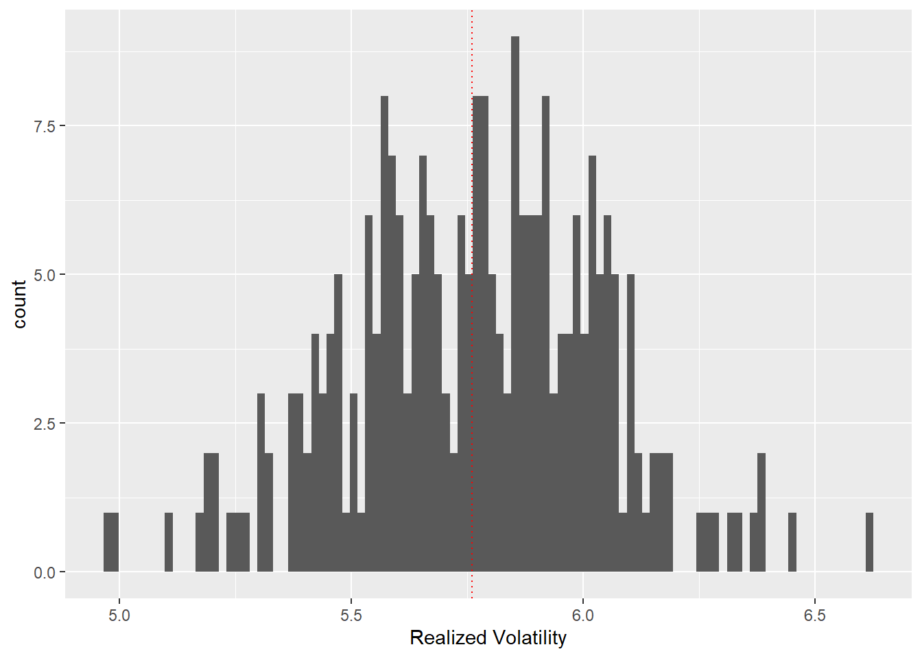
What about the realized volatility? As defined in the lecture, the realized variance \[RV = \sum\limits_{i=0}^n \Delta X_t^2\] converges to the integrated variance (in the absence of jumps). The bar plot below illustrates the sampling distribution of the realized volatility, which, as expected, centers around true_sigma, the integrated variance of the simulated geometric Brownian motion. You can change the value true_sigma above and analyze the effect.
Figure 6: Sampling distribution of the realized variance across 250 simulated GBM paths; the dotted vertical line marks the true integrated variance.
Finally, some more analysis regarding the infill asymptotics. As should be clear by now, sampling at the highest frequency possible will ensure that the realized volatility recovers the integrated variance of the (log) price process. In other words, we can measure the variance. The following lines of code illustrate the effect: Whereas we simulated our process at a high frequency, we now simulate sub-samples at different frequencies, ranging from every second to once per day. The figure then illustrates the daily realized volatilities relative to the integrated variance of the process. Not surprisingly, the dispersion around the true parameter decreases substantially with higher sampling frequency.
Note that the code below illustrates how to work with the xts package and switch between the tidyverse and the high-frequency data format requirements. Of course, the procedure could be more convenient, but it is worth exploiting the functionalities of both worlds instead of recording everything in a tidy manner.
import numpy as npimport pandas as pdfrom plotnine import*from datetime import datetime, timedeltaimport matplotlib.pyplot as pltplt.switch_backend("Agg")
First, the function below is a rather general version of a simulated generalized Brownian motion. Note that there is no immediate need to assign trading date and hour; I implement this because it will provide output closer to actual data, and therefore, parts of my code can be recycled for future projects. The function can be called with a specific seed to replicate the results. The relevant parameters are the initial values start and the geometric Brownian motion mu and sigma parameters. The input steps defines the simulated Brownian motion’s granularity (sampling frequency).
Note the last line of the function doing most of the work: We exploit that increments of a Brownian motion are independent and normally distributed. The entire path is nothing but the cumulative sum of the increments.
Next, I simulate the stock price with 1000 intraday observations. Recall that the geometric Brownian motion implies dynamics for the log of the stock price, which is why I adjust the plotted value in the \(y\)-axis.
<plotnine.ggplot.ggplot object at 0x0000023375AECCD0>
Next, we scale the simulation up. The code below simulates 250 paths of the geometric Brownian motion, all with the same starting value. The function illustrates the sampled (log) price paths.
<plotnine.ggplot.ggplot object at 0x00000233FCDBA850>
Next, we investigate some of the properties of the geometric Brownian motion. First, by definition, the sample variation of \(X_t = \int\limits_0^t\mu dt + \int\limits_0^t\sigma dW_t\) is \(\int\limits_0^t\sigma^2 dt = \sigma^2t\). The figure below illustrates the sample variation over time and shows that the standard deviation across all simulated (log) prices increases linearly in \(t\) as expected. For the simulation, I used \(\sigma = 2.4\) (true_sigma), which corresponds to the slope of the line (adjusted by the number of observations).
<plotnine.ggplot.ggplot object at 0x0000023377014990>
What about the realized volatility? As defined in the lecture, the realized variance \[RV = \sum\limits_{i=0}^n \Delta X_t^2\] converges to the integrated variance (in the absence of jumps). The bar plot below illustrates the sampling distribution of the realized volatility, which, as expected, centers around true_sigma, the integrated variance of the simulated geometric Brownian motion. You can change the value true_sigma above and analyze the effect.
<plotnine.ggplot.ggplot object at 0x0000023375954D10>
Finally, some more analysis regarding the infill asymptotics. As should be clear by now, sampling at the highest frequency possible will ensure that the realized volatility recovers the integrated variance of the (log) price process. In other words, we can measure the variance. The following lines of code illustrate the effect: Whereas we simulated our process at a high frequency, we now simulate sub-samples at different frequencies, ranging from every second to once per day. The figure then illustrates the daily realized volatilities relative to the integrated variance of the process. Not surprisingly, the dispersion around the true parameter decreases substantially with higher sampling frequency.