library(tidyverse)
library(tidyfinance)(Co)variance estimation
ARCH and GARCH
This short exercise illustrates how to perform maximum likelihood estimation using the simple example of ARCH\((p)\) and GARCH(\(p, q\)) models. First, write the code for the basic specification independently. Afterward, the exercises will help you familiarize yourself with well-established packages that provide the same (and much more sophisticated) methods to estimate conditional volatility models.
Exercises:
- As a benchmark dataset, download prices and compute daily returns for all stocks that are part of the Dow Jones 30 index. The sample period should start on January 1st, 2000. Then, decompose the time series into a predictable part and a residual, \(r_t = E(r_t|\mathcal{F}_{t-1}) + \varepsilon_t\). The most straightforward approach is to demean the series by subtracting the sample mean, but in principle more sophisticated methods (e.g. a factor model) can be used.
- For each of the 30 tickers, illustrate the rolling-window standard deviation based on an estimation window length of your choice.
- Write a small function that computes the maximum likelihood estimator (MLE) of an ARCH(\(p\)) model.
- Write a second function that implements MLE estimation for a GARCH(\(p,q\)) model.
- What is the unconditional estimated variance implied by the ARCH(\(1\)) and GARCH(\(1, 1\)) models for each ticker?
Solutions:
import pandas as pd
import numpy as np
import tidyfinance as tf
from plotnine import *
from scipy.optimize import minimize
As usual, I download daily prices for the 30 index constituents and compute (adjusted) net returns. I then demean each return series. This simple demeaning step could be replaced by adjusting returns with an estimated factor model or with predictions from the Machine Learning part of the course.
ticker <- download_data(
  type = "constituents",
  index = "Dow Jones Industrial Average"
) |> pull(symbol)
Warning: The `type` argument of `download_data()` is deprecated as of tidyfinance 0.5.0.
ℹ Use the `domain` and `dataset` arguments instead.Warning: The `type` argument of `download_data()` is deprecated as of tidyfinance 0.5.0.
ℹ Column type should be replaced with domain and dataset. Use
`list_supported_types()` to see the mapping.index_prices <- download_data(
type = "stock_prices",
symbols = ticker,
start_date = "2000-01-01"
)
returns <- index_prices |>
group_by(symbol) |>
mutate(ret = 100 * (adjusted_close / lag(adjusted_close) - 1)) |>
select(symbol, date, ret) |>
drop_na(ret) |>
mutate(ret = ret - mean(ret))tickers = (
tf.download_data(domain="constituents", index="Dow Jones Industrial Average")
)["symbol"].tolist()
index_prices = tf.download_data(
domain="stock_prices", symbols=tickers, start_date="2000-01-01"
)
returns = (
index_prices.sort_values(["symbol", "date"])
.groupby("symbol", group_keys=False)
.apply(
lambda df: df.assign(
ret=100 * (df["adjusted_close"] / df["adjusted_close"].shift(1) - 1)
)
)[["symbol", "date", "ret"]]
.dropna(subset=["ret"])
)
returns["ret"] = returns.groupby("symbol")["ret"].transform(lambda x: x - x.mean())As in the chapter on beta estimation, I use a rolling-window approach to compute the standard deviation. Requiring a complete window ensures that a rolling standard deviation is only reported once enough observations are available.
library(slider)

rolling_sd <- returns |>
  group_by(symbol) |>
  mutate(rolling_sd = slide_dbl(ret, sd,
                                .before = 100,
                                .complete = TRUE)) # 100 day estimation window

rolling_sd |>
  drop_na() |>
  ggplot(aes(x=date,
             y = sqrt(250) * rolling_sd,
             color = symbol)) +
  geom_line() +
  labs(x = "", y = "Standard deviation (annualized)") +
  theme(legend.position = "None")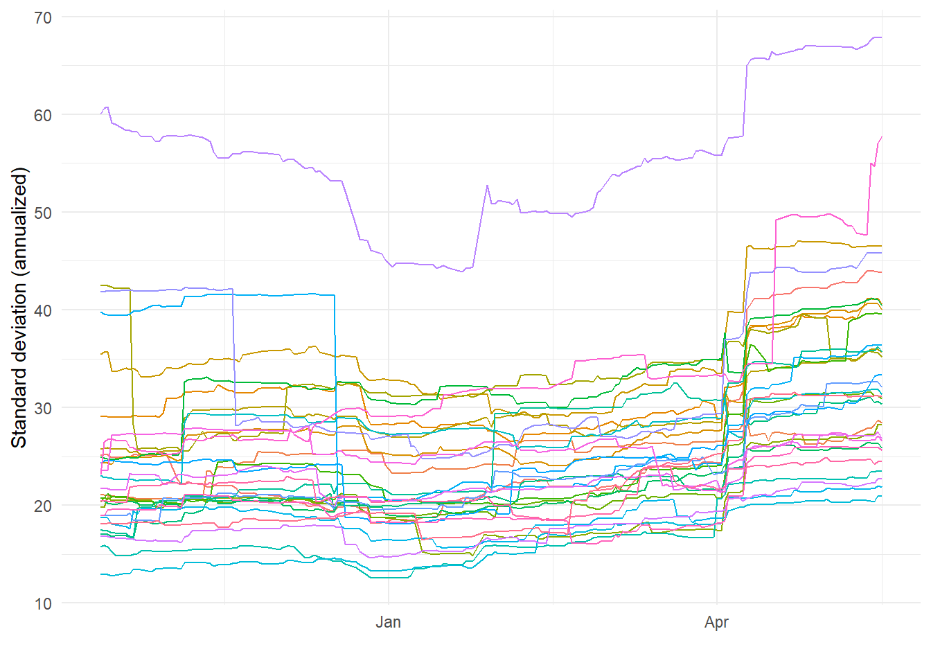
rolling_sd = returns.groupby("symbol", group_keys=False).apply(
    lambda df: df.assign(
        rolling_sd=df["ret"].rolling(window=101, min_periods=101).std()
    )
)

rolling_sd = rolling_sd.dropna(subset=["rolling_sd"]).assign(
    annualized_sd=np.sqrt(250) * rolling_sd["rolling_sd"]
)


(
    ggplot(rolling_sd, aes(x="date", y="annualized_sd", color="symbol"))
    + geom_line()
    + labs(x="", y="Standard deviation (annualized)")
    + theme(legend_position="none")
)
The figure illustrates two relevant stylized facts: i) volatilities are persistent but clearly change over time, and ii) volatilities tend to co-move across stocks. Next, I write a simplified routine that performs maximum likelihood estimation of an ARCH(\(p\)) model under Gaussian innovations.
logL_arch <- function(params, p, ret){
  # Inputs: params (a p + 1 x 1 vector of ARCH parameters)
  #         p (lag-length)
  #         ret demeaned returns
  # Output: the log-likelihood (for normally distributed innovation terms)
  eps_sqr_lagged <- cbind(ret, 1)
  for(i in 1:p){
    eps_sqr_lagged <- cbind(eps_sqr_lagged, lag(ret, i)^2)
  }
  eps_sqr_lagged <- na.omit(eps_sqr_lagged)
  sigma <- eps_sqr_lagged[,-1] %*% params
  if(any(sigma <= 0)) return(1e10)
  log_likelihood <- 0.5 * sum(log(sigma)) + 0.5 * sum(eps_sqr_lagged[,1]^2/sigma)
  return(log_likelihood)
}
def logL_arch(params, p, ret):
"""
Inputs: params (a p + 1 x 1 vector of ARCH parameters)
p (lag-length)
ret demeaned returns
Output: the log-likelihood (for normally distributed innovation terms)
"""
ret = np.asarray(ret)
X = np.column_stack(
[np.ones(len(ret))] + [np.roll(ret, i) ** 2 for i in range(1, p + 1)]
)
X = X[p:]
ret_clean = ret[p:]
sigma = X @ params
return 0.5 * np.sum(np.log(sigma)) + 0.5 * np.sum((ret_clean**2) / sigma)The function logL_arch computes the (log) likelihood of an ARCH specification with \(p\) lags. It returns the negative log-likelihood because the optimizers used below (optim in R, scipy.optimize.minimize in Python) search for minima.
The following lines estimate the model on demeaned AAPL returns (in percent) with \(p = 2\) lags. Note the (almost) arbitrary choice of initial parameter vector. Also note that neither logL_arch nor the optimizer enforces the regularity conditions that would guarantee a stationary volatility process.
p <- 2
ret <- returns |> filter(symbol == "AAPL") |> pull(ret)

initial_params <- c(var(ret), rep(1, p))
fit_manual <- optim(par = initial_params,
                    fn = logL_arch,
                    hessian = TRUE,
                    method="L-BFGS-B",
                    lower = 0,
                    p = p,
                    ret = ret)

fitted_params <- (fit_manual$par)
se <- sqrt(diag(solve(fit_manual$hessian)))

cbind(fitted_params, se) |> knitr::kable(digits = 2)| fitted_params | se |
|---|---|
| 2.58 | 0.29 |
| 0.40 | 0.12 |
| 0.00 | 0.04 |
# Run the code below to compare the results with tseries package
# library(tseries)
# summary(garch(ret,c(0,p)))
p = 2
ret = returns.loc[returns["symbol"] == "AAPL", "ret"].values
initial_params = np.concatenate(([np.var(ret, ddof=1)], np.ones(p)))
res = minimize(
logL_arch,
initial_params,
args=(p, ret),
bounds=[(0, None)] * (p + 1),
method="L-BFGS-B",
)
fitted_params = res.x
hessian_inv = res.hess_inv.todense()
se = np.sqrt(np.diag(hessian_inv))
pd.DataFrame({"param": fitted_params.round(2), "se": se.round(2)})GARCH estimation only requires a few adjustments to the ARCH code.
logL_garch <- function(params, p, q, ret,
                       return_only_loglik = TRUE){
  eps_sqr_lagged <- cbind(ret, 1)
  for(i in 1:p){
    eps_sqr_lagged <- cbind(eps_sqr_lagged, lag(ret, i)^2)
  }
  sigma.sqrd <- rep(sd(ret)^2, nrow(eps_sqr_lagged))
  for(t in (1 + max(p, q)):nrow(eps_sqr_lagged)){
    sigma.sqrd[t] <- params[1:(1+p)]%*% eps_sqr_lagged[t,-1] +
              params[(2+p):length(params)] %*% sigma.sqrd[(t-1):(t-q)]
  }
  sigma.sqrd <- sigma.sqrd[-(1:(max(p, q)))]
  if(any(sigma.sqrd <= 0)) return(1e10)

  if(return_only_loglik){
    0.5 * sum(log(sigma.sqrd)) + 0.5 * sum(eps_sqr_lagged[(1 + max(p, q)):nrow(eps_sqr_lagged),1]^2/sigma.sqrd)
  }else{
    return(sigma.sqrd)
  }
}

p <- 1 # Lag structure
q <- 1
fit_garch_manual <- optim(par = rep(0.01, p + q + 1),
                    fn = logL_garch,
                    hessian = TRUE,
                    method="L-BFGS-B",
                    lower = 0,
                    p = p,
                    q = q,
                    ret = ret)

fitted_garch_params <- fit_garch_manual$par
def logL_garch(params, p, q, ret, return_only_loglik=True):
ret = np.asarray(ret)
n = len(ret)
eps_sqr_lagged = np.column_stack([ret, np.ones(n)])
for i in range(1, p + 1):
lagged = np.empty(n)
lagged[:] = np.nan
lagged[i:] = ret[:-i]
eps_sqr_lagged = np.column_stack([eps_sqr_lagged, lagged**2])
sigma_sq = np.full(n, np.var(ret, ddof=1))
for t in range(max(p, q), n):
omega_alpha = params[: (1 + p)]
beta = params[(1 + p) :]
sigma_lags = np.array([sigma_sq[t - j] for j in range(1, q + 1)])
sigma_sq[t] = np.dot(omega_alpha, eps_sqr_lagged[t, 1:]) + np.dot(
beta, sigma_lags
)
start = max(p, q)
sigma_sq = sigma_sq[start:]
eps = eps_sqr_lagged[start:, 0]
mask = ~np.isnan(eps)
sigma_sq = sigma_sq[mask]
eps = eps[mask]
if return_only_loglik:
return 0.5 * np.sum(np.log(sigma_sq)) + 0.5 * np.sum((eps**2) / sigma_sq)
else:
return sigma_sq
p = 1
q = 1
init_params = np.full(p + q + 1, 0.01)
result = minimize(
logL_garch,
init_params,
args=(p, q, ret, True),
method="L-BFGS-B",
bounds=[(0, None)] * (p + q + 1),
)
fitted_garch_params = result.xNext, I plot the time series of the estimated conditional volatilities \(\sigma_t\) based on the fitted parameters. To keep the code compact, logL_garch returns the fitted variances when called with return_only_loglik = FALSE.
tibble(vola = logL_garch(fitted_garch_params, p, q, ret, FALSE)) |>
  ggplot(aes(x = 1:length(vola), y = sqrt(vola))) +
  geom_line() +
  labs(x = "", y  = "GARCH(1,1) volatility")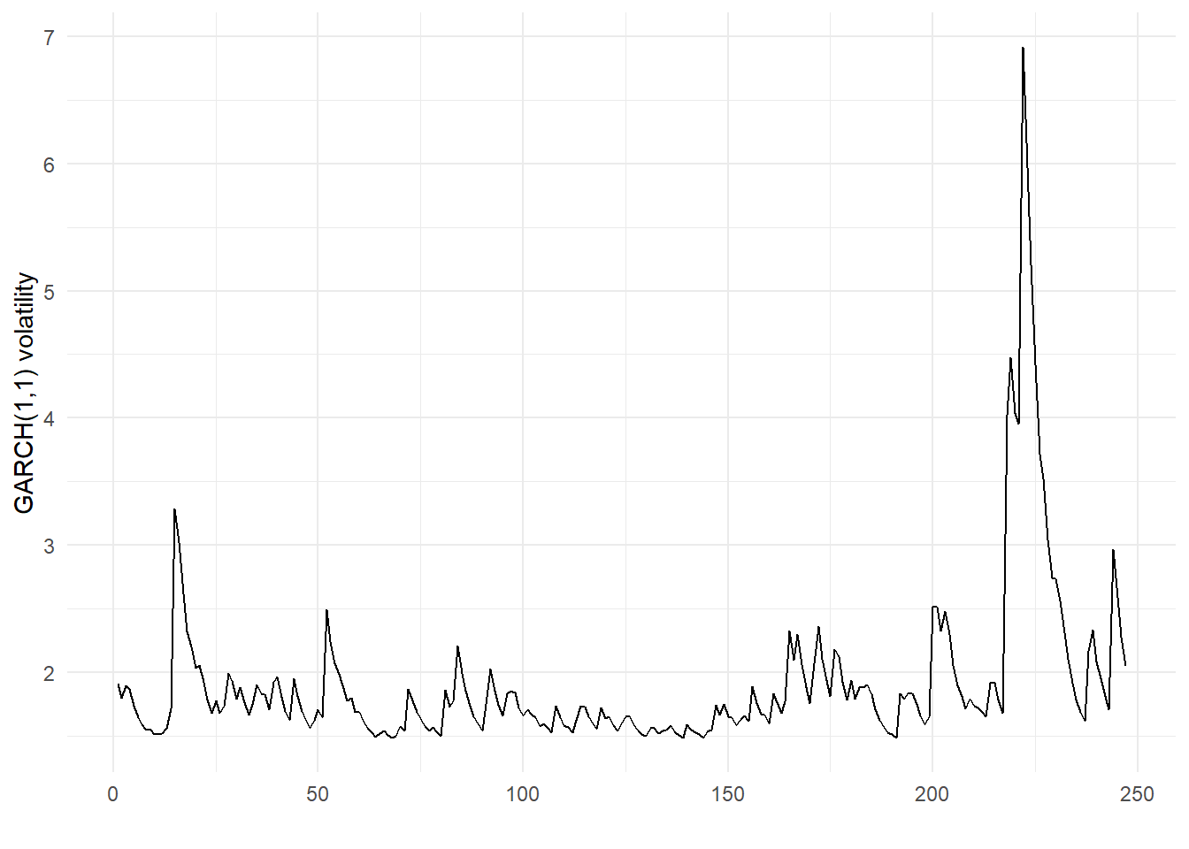
vola = logL_garch(fitted_garch_params, p, q, ret, False)
vola_date = np.arange(0, len(vola))
vola_df = pd.DataFrame({"date": vola_date, "vola": np.sqrt(vola)})

(
    ggplot(vola_df, aes(x="date", y="vola"))
    + geom_line()
    + labs(x="", y="GARCH(1,1) volatility")
    + theme(legend_position="none")
)
Once we have implemented the workflow for one asset, we can apply it to all assets in the sample — using mutate() together with map() in R, or a groupby loop in Python. The lecture slides define the unconditional variance implied by the ARCH model.
unconditional_volatility <- returns |>
  arrange(symbol, date) |>
  nest(data = c(date, ret)) |>
  mutate(arch = map(data, function(.x){

    ret <- .x |> pull(ret)
    p <- 1
    initial_params <- c(var(ret), rep(1, p))
    fit_manual <- optim(par = initial_params,
                        fn = logL_arch,
                        hessian = TRUE,
                        method="L-BFGS-B",
                        lower = 0,
                        p = p,
                        ret = ret)

    fitted_params <- fit_manual$par
    se <- sqrt(diag(solve(fit_manual$hessian)))

    return(tibble(param = c("intercept", paste0("alpha_", 1:p)),
                  value = fitted_params, se = se))
  })) |>
  select(-data) |>
  unnest(arch) |>
  group_by(symbol) |>
  summarise(uncond_var = dplyr::first(value) / (1 - sum(value) + dplyr::first(value))) |>
  ungroup()

unconditional_volatility |>
  ggplot() +
  geom_bar(aes(x = reorder(symbol, uncond_var),
               y = sqrt(250) * uncond_var), stat = "identity") +
  coord_flip() +
  labs(x = "Unconditional volatility (annualized)",
      y = "")
def compute_unconditional_volatility(returns):
results = []
for symbol, df in returns.sort_values(["symbol", "date"]).groupby("symbol"):
ret = df["ret"].values
p = 1
initial_params = np.concatenate([[np.var(ret, ddof=1)], np.ones(p)])
res = minimize(
logL_arch,
x0=initial_params,
args=(p, ret),
method="L-BFGS-B",
bounds=[(0, None)] * (p + 1),
)
fitted_params = res.x
try:
hess_inv = res.hess_inv.todense()
except:
hess_inv = res.hess_inv
se = np.sqrt(np.diag(hess_inv))
omega = fitted_params[0]
alpha_sum = np.sum(fitted_params[1:])
uncond_var = omega / (1 - alpha_sum)
results.append({"symbol": symbol, "uncond_var": uncond_var})
return pd.DataFrame(results)
unconditional_volatility = (
compute_unconditional_volatility(returns)
.assign(annualized_vol=lambda df: np.sqrt(250) * df["uncond_var"])
.sort_values("annualized_vol", ascending=False)
.assign(
symbol=lambda df: pd.Categorical(
df["symbol"], categories=df["symbol"][::-1], ordered=True
)
)
)
(
ggplot(unconditional_volatility)
+ geom_bar(aes(x="symbol", y="annualized_vol"), stat="identity")
+ coord_flip()
+ labs(x="Unconditional volatility (annualized)", y="")
)Ledoit-Wolf shrinkage estimation
A severe practical issue with the sample variance-covariance matrix in large dimensions (\(N \gg T\)) is that \(\hat\Sigma\) becomes singular. Ledoit and Wolf proposed a family of biased estimators of \(\Sigma\) that overcome this problem. As a result, it is often advisable to apply Ledoit-Wolf-style shrinkage to the variance-covariance matrix before proceeding with portfolio optimization.
Exercises:
- Read the introduction of the paper Honey, I shrunk the sample covariance matrix and implement the feasible linear shrinkage estimator. If in doubt, consult Michael Wolf’s homepage, where you will find reference R and Python code.
- Write a simulation that generates iid returns of dimension \(T \times N\) (e.g., with
rnorm()in R ornp.random.randn()in Python) and compute the minimum-variance portfolio weights based on (i) the sample variance-covariance matrix and (ii) Ledoit-Wolf shrinkage. What is the mean squared deviation from the theoretically optimal portfolio (\(1/N\))? What can you conclude?
Solutions:
The exercise requires a thorough reading of the original paper — translating the derivations into working code is non-trivial. The reference implementations below can serve as a starting point for future assignments. Note that compute_ledoit_wolf expects a \(T \times N\) input matrix, where rows index time periods and columns index assets. Passing the transposed matrix is a common source of errors.
compute_ledoit_wolf <- function(x) {
  # Computes Ledoit-Wolf shrinkage covariance estimator
  # This function generates the Ledoit-Wolf covariance estimator  as proposed in Ledoit, Wolf 2004 (Honey, I shrunk the sample covariance matrix.)
  # X is a (t x n) matrix of returns
  t <- nrow(x)
  n <- ncol(x)
  x <- apply(x, 2, function(x) if (is.numeric(x)) # demean x
    x - mean(x) else x)
  sample <- (1/t) * (t(x) %*% x)
  var <- diag(sample)
  sqrtvar <- sqrt(var)
  rBar <- (sum(sum(sample/(sqrtvar %*% t(sqrtvar)))) - n)/(n * (n - 1))
  prior <- rBar * sqrtvar %*% t(sqrtvar)
  diag(prior) <- var
  y <- x^2
  phiMat <- t(y) %*% y/t - 2 * (t(x) %*% x) * sample/t + sample^2
  phi <- sum(phiMat)

  repmat = function(X, m, n) {
    X <- as.matrix(X)
    mx = dim(X)[1]
    nx = dim(X)[2]
    matrix(t(matrix(X, mx, nx * n)), mx * m, nx * n, byrow = T)
  }

  term1 <- (t(x^3) %*% x)/t
  help <- t(x) %*% x/t
  helpDiag <- diag(help)
  term2 <- repmat(helpDiag, 1, n) * sample
  term3 <- help * repmat(var, 1, n)
  term4 <- repmat(var, 1, n) * sample
  thetaMat <- term1 - term2 - term3 + term4
  diag(thetaMat) <- 0
  rho <- sum(diag(phiMat)) + rBar * sum(sum(((1/sqrtvar) %*% t(sqrtvar)) * thetaMat))

  gamma <- sum(diag(t(sample - prior) %*% (sample - prior)))
  kappa <- (phi - rho)/gamma
  shrinkage <- max(0, min(1, kappa/t))
  if (is.nan(shrinkage))
    shrinkage <- 1
  sigma <- shrinkage * prior + (1 - shrinkage) * sample
  return(sigma)
}
def compute_ledoit_wolf(x):
"""
Computes Ledoit-Wolf shrinkage covariance estimator
This function generates the Ledoit-Wolf covariance estimator as proposed in Ledoit, Wolf 2004 (Honey, I shrunk the sample covariance matrix.)
X is a (t x n) matrix of returns
"""
x = np.asarray(x)
t, n = x.shape
x = x - np.mean(x, axis=0)
sample = (1 / t) * (x.T @ x)
var = np.diag(sample)
sqrtvar = np.sqrt(var)
denom = np.outer(sqrtvar, sqrtvar)
rBar = (np.sum(sample / denom) - n) / (n * (n - 1))
prior = rBar * denom
np.fill_diagonal(prior, var)
y = x**2
phiMat = (y.T @ y) / t - 2 * (x.T @ x) * sample / t + sample**2
phi = np.sum(phiMat)
def repmat(X, m, n):
return np.tile(X, (m, n))
term1 = ((x**3).T @ x) / t
help_mat = (x.T @ x) / t
helpDiag = np.diag(help_mat)
term2 = repmat(helpDiag.reshape(-1, 1), 1, n) * sample
term3 = help_mat * repmat(var.reshape(-1, 1), 1, n)
term4 = repmat(var.reshape(-1, 1), 1, n) * sample
thetaMat = term1 - term2 - term3 + term4
np.fill_diagonal(thetaMat, 0)
rho = np.sum(np.diag(phiMat)) + rBar * np.sum(
(np.outer(1 / sqrtvar, sqrtvar)) * thetaMat
)
gamma = np.trace((sample - prior).T @ (sample - prior))
kappa = (phi - rho) / gamma
shrinkage = max(0, min(1, kappa / t))
if np.isnan(shrinkage):
shrinkage = 1
sigma = shrinkage * prior + (1 - shrinkage) * sample
return sigmaThe simulation is structured as follows. The helper functions simulate an iid normal “returns” matrix for given dimensions T and N, and then compute minimum-variance portfolio weights using either the sample variance-covariance matrix or its Ledoit-Wolf shrinkage counterpart. Setting a seed via set.seed() (R) or np.random.seed() (Python) ensures the random draws — and therefore the results — are reproducible.
set.seed(2023)

generate_returns <- function(T, N) matrix(rnorm(T * N), nc = N)

# Minimum variance portfolio weights
compute_mvp_sample <- function(mat){
  w <- solve(cov(mat))%*% rep(1,ncol(mat))
  return(w/sum(w))
}
compute_mvp_lw <- function(mat){
  w <- solve(compute_ledoit_wolf(mat))%*% rep(1,ncol(mat))
  return(w/sum(w))
}

eval_weight <- function(w) length(w)^2 * sum((w - 1/length(w))^2)np.random.seed(2023)
def generate_returns(T, N):
return np.random.randn(T, N)
def compute_mvp_sample(mat):
w = np.linalg.solve(np.cov(mat, rowvar=False), np.ones(mat.shape[1]))
return w / np.sum(w)
def compute_mvp_lw(mat):
w = np.linalg.solve(compute_ledoit_wolf(mat), np.ones(mat.shape[1]))
return w / np.sum(w)
def eval_weight(w):
n = len(w)**2
return n * np.sum((w - 1 / n) ** 2)I evaluate the estimated weights based on their squared deviation from the naive \(1/N\) portfolio, which is the true minimum-variance portfolio under iid returns. The scaling factor \(N^2\) is included to penalize errors more heavily in higher dimensions.
simulation <- function(T = 100, N = 70){
  simulation_rounds <- 50
  tmp <- matrix(NA, nc = 2, nr = simulation_rounds)
  for(i in 1:simulation_rounds){
    mat <- generate_returns(T, N)
    w_lw <- compute_mvp_lw(mat)
    if(N < T) w_sample <- compute_mvp_sample(mat)
    if(N >= T) w_sample <- rep(NA, N)
    tmp[i, 1] <- eval_weight(w_lw)
    tmp[i, 2] <- eval_weight(w_sample)
  }
  tibble(model = c("Shrinkage", "Sample"), error = colMeans(tmp), N = N, T = T)
}

result <- bind_rows(simulation(100, 60),
                    simulation(100, 70),
                    simulation(100, 80),
                    simulation(100, 90),
                    simulation(100, 100),
                    simulation(100, 150))

result |>
  pivot_wider(names_from = model, values_from = error) |>
knitr::kable(digits = 2, "pipe")| N | T | Shrinkage | Sample |
|---|---|---|---|
| 60 | 100 | 1.30 | 89.59 |
| 70 | 100 | 1.51 | 164.15 |
| 80 | 100 | 1.60 | 305.91 |
| 90 | 100 | 1.99 | 874.19 |
| 100 | 100 | 2.23 | NA |
| 150 | 100 | 3.29 | NA |
def simulation(T=100, N=70):
    simulation_rounds = 50
    tmp = np.full((simulation_rounds, 2), np.nan)

    for i in range(simulation_rounds):
        mat = generate_returns(T, N)
        w_lw = compute_mvp_lw(mat)

        if N < T:
            w_sample = compute_mvp_sample(mat)
        else:
            w_sample = np.full(N, np.nan)

        tmp[i, 0] = eval_weight(w_lw)
        tmp[i, 1] = eval_weight(w_sample)

    return pd.DataFrame(
        {
            "model": ["Shrinkage", "Sample"],
            "error": np.nanmean(tmp, axis=0),
            "N": N,
            "T": T,
        }
    )

result = pd.concat(
    [
        simulation(100, 60),
        simulation(100, 70),
        simulation(100, 80),
        simulation(100, 90),
        simulation(100, 100),
        simulation(100, 150),
    ],
    ignore_index=True,
)

result_pivot = result.pivot(index=["N", "T"], columns="model", values="error")

print(result_pivot.round(2))
The results highlight two takeaways. First, the sample variance-covariance matrix breaks down once \(N \geq T\): it is no longer invertible, so a unique minimum-variance portfolio does not exist. Ledoit-Wolf-style shrinkage, by contrast, remains positive definite even when \(N > T\). Second, the (scaled) mean squared error of the portfolio weights relative to the optimal naive portfolio is substantially smaller for the shrinkage estimator. Although the shrinkage estimator is biased, its variance is reduced enough to deliver markedly more robust portfolio weights.